Portfolio Allocation Models
The aim of portfolio allocation is to construct a portfolio by determining the proportions of our portfolio that each asset should hold, according to quantifiable characteristics such as risk, return, covariance matrices, as well as mathematical methodologies such as optimization (i.e. CLA) and machine learning techniques (i.e. hierarchical clustering).
Let’s use the Dow Jones Industrial Average as our market proxy. It will be our main use case throughout this tutorial.
>>> # Construct the DJIA index portfolio
>>> market_portfolio = Portfolio(assets='^DJI')
>>> market_portfolio.set_frequency(frequency='M', inplace=True) # resample to Monthly
>>> market_portfolio.slice_dataframe(from_date=datetime(2016, 1, 1), to_date=datetime(2020, 1, 1), inplace=True)
>>> # Construct the DJIA constituents portfolio
>>> assets = macro.companies_in_index(MarketIndices.DOW_JONES)
>>> portfolio = Portfolio(assets=assets)
>>> portfolio.set_frequency(frequency='M', inplace=True)
>>> portfolio.slice_dataframe(from_date=datetime(2016, 1, 1), to_date=datetime(2020, 1, 1), inplace=True)
>>> print(portfolio.df_returns.tail(10))
                          MMM       AXP      AMGN  ...       WBA       WMT       DIS
Date                                               ...
2019-03-31 23:59:59  0.001881  0.014479 -0.000526  ... -0.111251 -0.009448 -0.016040
2019-04-30 23:59:59 -0.087929  0.076349 -0.056111  ... -0.153311  0.054445  0.233631
2019-05-31 23:59:59 -0.149824 -0.021496 -0.062373  ... -0.071178 -0.008374 -0.035993
2019-06-30 23:59:59  0.085070  0.076105  0.105459  ...  0.108026  0.089215  0.057558
2019-07-31 23:59:59  0.007961  0.010685  0.012481  ... -0.003292 -0.000996  0.030476
2019-08-31 23:59:59 -0.065935 -0.032162  0.126048  ... -0.051960  0.040247 -0.040207
2019-09-30 23:59:59  0.016572 -0.017363 -0.072428  ...  0.080484  0.038684 -0.050561
2019-10-31 23:59:59  0.003589 -0.004662  0.102010  ... -0.009582 -0.011965 -0.003069
2019-11-30 23:59:59  0.037880  0.024216  0.107994  ...  0.096093  0.015606  0.166718
2019-12-31 23:59:59  0.039171  0.036380  0.027054  ... -0.010738  0.002377 -0.040134
[10 rows x 30 columns]
Modern Portfolio Theory
In a 1952 essay, economist Harry Markowitz introduced Modern Portfolio Theory (MPT). Also termed mean-variance analysis, it is a mathematical framework for determining the proportion of an asset in the portfolio, so that the expected return is maximized for a given level of risk. It formalizes the idea of diversification, i.e. that owning different types of financial assets is less risky than owning only one. Essentially, an asset’s risk and return should not be assessed by itself, but by how it contributes to the risk and overall return of a portfolio.
Markowitz Mean-Variance Framework (1952)
>>> MPT = ModernPortfolioTheory(portfolio)
>>> weights = MPT.solve_weights(use_sharpe=True)
>>> print(weights)
MMM     8.252014e-11
AXP     5.754070e-12
AMGN    1.026955e-11
AAPL    1.065381e-09
BA      0.000000e+00
CAT     5.458483e-11
CVX     1.986690e-11
CSCO    3.633562e-11
KO      4.627803e-01
DOW     5.289753e-12
GS      4.808235e-11
HD      1.116429e-11
HON     0.000000e+00
IBM     8.356778e-12
INTC    8.504801e-12
JNJ     1.047248e-11
JPM     1.002877e-02
MCD     0.000000e+00
MRK     0.000000e+00
MSFT    0.000000e+00
NKE     0.000000e+00
PG      5.280897e-02
CRM     2.149651e-11
TRV     5.207088e-02
UNH     1.965341e-01
VZ      0.000000e+00
V       2.266829e-12
WBA     0.000000e+00
WMT     2.257769e-01
DIS     0.000000e+00
dtype: float64
Efficient Frontier
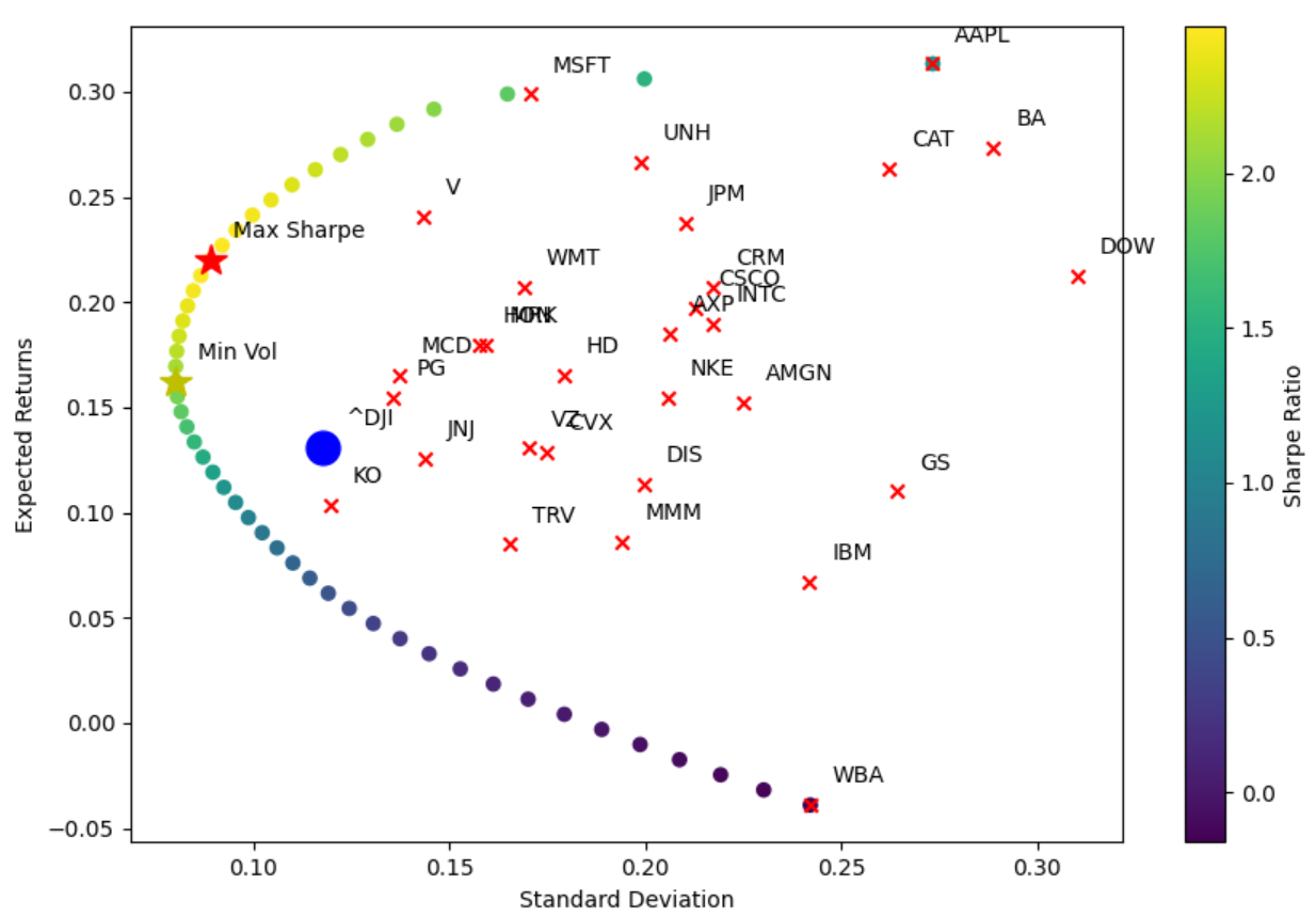
>>> stats_df = MPT.markowitz_efficient_frontier(market_portfolio=market_portfolio, plot_assets=True, plot_cal=True)
>>> pd.set_option('display.max_columns', None) # show all columns
>>> print(stats_df.head())
   Target Return  Minimum Volatilty  Sharpe Ratio  \
0      -0.038987           0.242079     -0.161053
1      -0.031797           0.230182     -0.138139
2      -0.024607           0.219190     -0.112263
3      -0.017417           0.208682     -0.083460
4      -0.010226           0.198630     -0.051484
                                     Optimal Weights
0  [0.0, 5.676814812498321e-17, 6.248307942010797...
1  [0.0, 2.1251952869548186e-16, 7.33663515761706...
2  [1.0495623187945156e-16, 1.022455433619923e-16...
3  [0.0, 0.0, 2.0295223730939766e-16, 0.0, 1.3976...
4  [1.7626656648200915e-16, 1.4969544279368077e-1...
The resulting graph follows:
Capital Allocation Line
The tangent to the upper part of the hyperbolic boundary is the Capital Allocation Line (CAL), determining how to allocate funds between a risky asset and a risk-free asset. It is given by the equation:
where \(P\) is the sub-portfolio of risky assets at the tangency with the Markowitz bullet, \(F\) is the risk-free asset, and \(C\) is a combination of portfolios \(P\) and \(F\). It is also known as the Capital Market Line (CML).
Security Market Line
The Security Market Line (SML)
Capital Asset Pricing Model
As we’ve seen in the Asset Pricing Models module, the CAPM states that the expected return of any given asset should equal \(R_i = R_f + \beta_i * (R_m - R_f)\), with \(\alpha\) being the error term having an expected value of zero in theory. Thus, the only way to achieve higher expected returns is taking on more \(\beta\) (given that \((R_m - R_f) > 0\)). Every individual stock has some idiosyncratic risk in addition to its market \(\beta\) (true always when correlated less than perfectly with the market).
Note
The total risk is a combination of systematic and unsystematic (idiosyncratic) risk. * Systematic risk is given by the estimated coefficient of a regression of a security on a market portfolio,
\(\beta_{security, market} = \frac{\sigma_{security, market}}{\sigma_{market}^2}\).
The idiosyncratic risk is the portion of risk unexplained by the market factor, \(1 - R^2\). Empirically, the idiosyncratic risk in a single-factor contemporaneous CAPM model with US equities is around 60-70%.
Through diversification (i.e. by the mean-variance optimization process), unsystematic risk is eliminated. Thus, we can get the best return/risk ratio by buying the market portfolio, as buying anything else, we could not get more expected return for the same \(\beta\), but would only get some additional idiosyncratic risk.
To maximize investor’s utility function, Modern Portfolio Theory suggests holding the combination of a risk-free asset and optimal risky portfolio (ORP) lying on a tangency of the efficient frontier and capital market line. Modern Portfolio Theory also suggests that optimal risky portfolio is a market portfolio (e.g. capitalization-weighted index).
If we assume markets are fully efficient and all assets are fairly priced, we don’t have any reason to deviate from the market portfolio in our asset allocation. In such case, we don’t even need to know equilibrium asset returns nor perform any kind of portfolio optimization. An optimization based on equilibrium asset returns would lead back to the same market portfolio anyway.
Note
Using historical data to estimate expected returns implies nonzero expected \(\alpha\)-s for all assets. This is not coherent with the CAPM framework, so using this methodology within MPT, it has nothing to do with CAPM. In effect by using MPT this way, you are generating a momentum based investment strategy, as you assume that assets that have had good returns historically will continue to have good returns in the future.
This framework has then been improved by other economists and mathematicians who went on to account for its limitations.
Treynor-Black Model (1973)
Unlike the Markowitz’s approach for portfolio allocation, the Treynor-Black model is a type of active portfolio management.
Black-Litterman Model (1990)
The Black–Litterman model optimization is an extension of unconstrained Markowitz optimization that incorporates relative and absolute ‘views’ on inputs of risk and returns from.
Post Modern Portfolio Theory (1991)
Post-modern portfolio theory extends MPT by adopting non-normally distributed, asymmetric, and fat-tailed measures of risk. Two major limitations of MPT are in measuring risk and return in a way that doesn’t represent the realities of the investment markets. Specifically, it assumes the following:
Risk proxy: The variance of portfolio returns is the correct measure of investment risk. Using the variance (or its square root, the standard deviation) implies that uncertainty about better-than-expected returns is equally averred as uncertainty about returns that are worse than expected. It has long been recognized that investors typically do not view as risky those returns above the minimum they must earn in order to achieve their investment objectives. They believe that risk has to do with the bad outcomes (i.e., returns below a required target), not the good outcomes (i.e., returns in excess of the target) and that losses weigh more heavily than gains.
Statistical distribution: The investment returns of all securities and portfolios can be adequately represented by a joint elliptical distribution, such as the normal distribution. The assumption of a normal distribution is a major practical limitation, because it is symmetrical. Using the normal distribution to model the pattern of investment returns makes investment results with more upside than downside returns appear more risky than they really are.
Recent advances in portfolio and financial theory, coupled with increased computing power, have overcome these limitations. The resulting expanded risk/return paradigm is known as Post-Modern Portfolio Theory, or PMPT. Thus, MPT becomes nothing more than a special (symmetrical) case of PMPT.
Note
The risk measures we will describe below are mainly used to evaluate mutual fund and portfolio manager performance. It is important to note that some variables will cause differing results, such as the frequency (daily, weekly, monthly, yearly) and the *window*(from which date to which date). For example, some services calculate ‘during the last 3 years, the 30 days X is Y’.
Also, regarding time horizon, if you have a mean for a horizon of say 10 days, and a volatility over a year, then you can convert that volatility to be over the horizon by multiplying by \(\sqrt{10/252}\).
As a case, let’s take as an example the following portfolio
>>> from portfolio_management.Portfolio import Portfolio
>>> from datetime import datetime
>>> assets = ['AAPL', 'V', 'KO', 'CAT']
>>> portfolio = Portfolio(assets=assets)
>>> portfolio.slice_dataframe(to_date=datetime(2021, 1, 1), from_date=datetime(2016, 1, 1))
>>> portfolio_returns = portfolio.get_weighted_sum_returns(weights=np.ones(len(assets)) / len(assets))
>>> print(portfolio_returns.head())
Date
1970-01-05 23:59:59   -0.004553
1970-01-06 23:59:59   -0.003728
1970-01-07 23:59:59   -0.006211
1970-01-08 23:59:59    0.001179
1970-01-09 23:59:59   -0.005915
dtype: float64
First, we cover some measures that are based on the Capital Asset Pricing Model:
Risk Deviation Measures
Risk Adjusted Returns Measures Based on Volatility
Volatility is simply the average dispersion of the returns around their mean
>>> print(roys_safety_first_criterion(portfolio_returns=portfolio_returns, minimum_threshold=0.02, period=252))
0.7591708635828361
Value at Risk (VaR)
Measures of risk-adjusted return based on volatility treat all deviations from the mean as risk, whereas measures of risk-adjusted return based on lower partial moments consider only deviations below some predefined minimum return threshold, t as risk i.e. positive deviations aren’t risky. VaR is a more probabilistic view of loss as the risk of a portfolio
Risk Adjusted Returns Measures Based on VaR
Value at Risk computes the expected loss over a specified period of time given a confidence level
Drawdown Risk
Partial Moments Risk
These measures consider downside risk, and do not assume that returns are normally adjusted. The mean and variance do not completely describe the distribution, therefore using only both of them (i.e. the first and second moment of a distribution), would technically assume a normal distribution.